pandas

url_titanic = "https://gist.githubusercontent.com/butuzov/ed1c7f8f3affe6dd005c1ee40dc3f7f2/raw/87c7d72e009f1965263edc3431adbd4fab69f387/titanic.csv"
url_economics = "https://gist.githubusercontent.com/butuzov/ed1c7f8f3affe6dd005c1ee40dc3f7f2/raw/87c7d72e009f1965263edc3431adbd4fab69f387/economics.csv"
import pandas as pd
import numpy as np

import matplotlib.pyplot as plt
%matplotlib inline

# Just So we can log
# nice logging
from icecream import ic
import sys, re
def printError(e): print("Error: {}".format(e), file=sys.stderr)

def jupyter(*args):
    print(*[re.sub(r",\s{1,}", ", ", i.replace(",\n", ", ")) for i in args], file=sys.stdout)

ic.configureOutput(prefix='ic> ', outputFunction=jupyter)

rnd = np.random.RandomState(42)
Pandas
Talks:
Docks:
Books:
#Getting Started
pandas allow us plot, explore, data. perform math on large sets of it.
#Versions and general overview
# version
ic(pd.__version__)

> ic> pd.__version__: '1.5.3'

result >>> '1.5.3'
economics = pd.read_csv(url_economics, index_col='date',parse_dates=True)
economics.head(2)
|
pce |
pop |
psavert |
uempmed |
unemploy |
| date |
|
|
|
|
|
| 1967-07-01 |
507.4 |
198712 |
12.5 |
4.5 |
2944 |
| 1967-08-01 |
510.5 |
198911 |
12.5 |
4.7 |
2945 |
#Options
https://pandas.pydata.org/pandas-docs/stable/user_guide/options.html#available-options
ic(pd.describe_option("display.max_rows"))

with pd.option_context('display.max_rows', 2):
    ic(pd.get_option("display.max_rows"))
ic(pd.get_option("display.max_rows"))
print("----"*20)
ic(pd.get_option("display.max_rows"))
ic(pd.set_option("display.max_rows", 2))
ic(pd.get_option("display.max_rows"))
print("----"*20)
ic(pd.reset_option("display.max_rows"))
ic(pd.get_option("display.max_rows"))

> display.max_rows : int
> If max_rows is exceeded, switch to truncate view. Depending on
> `large_repr`, objects are either centrally truncated or printed as
> a summary view. 'None' value means unlimited.
>
> In case python/IPython is running in a terminal and `large_repr`
> equals 'truncate' this can be set to 0 and pandas will auto-detect
> the height of the terminal and print a truncated object which fits
> the screen height. The IPython notebook, IPython qtconsole, or
> IDLE do not run in a terminal and hence it is not possible to do
> correct auto-detection.
> [default: 60] [currently: 60]
> ic> pd.describe_option("display.max_rows"): None
> ic> pd.get_option("display.max_rows"): 2
> ic> pd.get_option("display.max_rows"): 60
> --------------------------------------------------------------------------------
> ic> pd.get_option("display.max_rows"): 60
> ic> pd.set_option("display.max_rows", 2): None
> ic> pd.get_option("display.max_rows"): 2
> --------------------------------------------------------------------------------
> ic> pd.reset_option("display.max_rows"): None
> ic> pd.get_option("display.max_rows"): 60

result >>> 60
#DataTypes: Series and DataFrames
Types:
np.bool (bool) - Stored as a single byte.np.int (int) - Defaulted to 64 bits, Unsigned ints is alaso available (np.uint)np.float (float) - Defaulted to 64 bits.np.complex (complex) - Rarely seen in DAnp.object (O, object) - Typically strings but is a catch- all for columns with multiple different types or other Python objects (tuples, lists, dicts, and so on).np.datetime64, pd.Timestamp (datetime64) - Specific moment in time with nanosecond precision.np.timedelta64,pd.Timedelta (timedelta64) - An amount of time, from days to nanoseconds.pd.Categorical (Categorical) - Specific only to pandas. Useful for object columns with relatively few unique values.
ic(economics.dtypes.value_counts())

print("-"*60)

ic(economics.dtypes)

> ic> economics.dtypes.value_counts(): float64    3
> int64      2
> dtype: int64
> ------------------------------------------------------------
> ic> economics.dtypes: pce         float64
> pop           int64
> psavert     float64
> uempmed     float64
> unemploy      int64
> dtype: object

result >>> pce         float64
result >>> pop           int64
result >>> psavert     float64
result >>> uempmed     float64
result >>> unemploy      int64
result >>> dtype: object
#pd.Series
numpy array with labels

rnd_series = pd.Series(rnd.randint(0, 10, 6))

ic(type(rnd_series))
ic(rnd_series.shape)
ic(rnd_series.index)
ic(rnd_series.value_counts(normalize=True))
ic(rnd_series.hasnans)

> ic> type(rnd_series): <class 'pandas.core.series.Series'>
> ic> rnd_series.shape: (6,)
> ic> rnd_series.index: RangeIndex(start=0, stop=6, step=1)
> ic> rnd_series.value_counts(normalize=True): 6    0.333333
> 3    0.166667
> 7    0.166667
> 4    0.166667
> 9    0.166667
> dtype: float64
> ic> rnd_series.hasnans: False

result >>> False
#pd.DataFrame
economics = pd.read_csv(url_economics, index_col='date',parse_dates=True)
economics.head(2)
|
pce |
pop |
psavert |
uempmed |
unemploy |
| date |
|
|
|
|
|
| 1967-07-01 |
507.4 |
198712 |
12.5 |
4.5 |
2944 |
| 1967-08-01 |
510.5 |
198911 |
12.5 |
4.7 |
2945 |
# row
ic(economics.values[0])
ic(type(economics.values))
ic(economics.shape)
ic(economics.columns[0:4])
ic(economics.index[0])

> ic> economics.values[0]: array([5.07400e+02, 1.98712e+05, 1.25000e+01, 4.50000e+00, 2.94400e+03])
> ic> type(economics.values): <class 'numpy.ndarray'>
> ic> economics.shape: (574, 5)
> ic> economics.columns[0:4]: Index(['pce', 'pop', 'psavert', 'uempmed'], dtype='object')
> ic> economics.index[0]: Timestamp('1967-07-01 00:00:00')

result >>> Timestamp('1967-07-01 00:00:00')
economics.info()

> <class 'pandas.core.frame.DataFrame'>
> DatetimeIndex: 574 entries, 1967-07-01 to 2015-04-01
> Data columns (total 5 columns):
> #   Column    Non-Null Count  Dtype
> ---  ------    --------------  -----
> 0   pce       574 non-null    float64
> 1   pop       574 non-null    int64
> 2   psavert   574 non-null    float64
> 3   uempmed   574 non-null    float64
> 4   unemploy  574 non-null    int64
> dtypes: float64(3), int64(2)
> memory usage: 26.9 KB
#Data: Generate Data (numpy)
pandas use numpy to generate indexes, and perform operations on matrixes
#Random data in Dataframe/Series
# generating random data based on numpy generated array
pd.DataFrame(rnd.randint(0, 10, 6).reshape(-1, 6)).head()
|
0 |
1 |
2 |
3 |
4 |
5 |
| 0 |
2 |
6 |
7 |
4 |
3 |
7 |
#Data: Import and Export
#Import
We can import data from: csv, excel, excel, hdfs, etc…
# Read a comma-separated values (csv) file into DataFrame.
economics = pd.read_csv(url_economics, index_col='date', parse_dates=True)
economics.head(3)
|
pce |
pop |
psavert |
uempmed |
unemploy |
| date |
|
|
|
|
|
| 1967-07-01 |
507.4 |
198712 |
12.5 |
4.5 |
2944 |
| 1967-08-01 |
510.5 |
198911 |
12.5 |
4.7 |
2945 |
| 1967-09-01 |
516.3 |
199113 |
11.7 |
4.6 |
2958 |
#Export
# excel export depends on openpyxl
#> pip install openpyxl 2>&1 1>/dev/null
>
> �[1m[�[0m�[34;49mnotice�[0m�[1;39;49m]�[0m�[39;49m A new release of pip is available: �[0m�[31;49m23.3.1�[0m�[39;49m -> �[0m�[32;49m23.3.2�[0m
> �[1m[�[0m�[34;49mnotice�[0m�[1;39;49m]�[0m�[39;49m To update, run: �[0m�[32;49mpip install --upgrade pip�[0m
# Write DataFrame to a comma-separated values (csv) file.
economics.to_csv(path_or_buf="data.csv", index=False)

# and actual saving dataframe to excel
economics.to_excel("data.xlsx")
#> unlink data.xlsx
#> unlink data.csv
#Export to data structures
dfdict = economics.to_dict()
ic(len(dfdict))
ic(dfdict.keys())

> ic> len(dfdict): 5
> ic> dfdict.keys(): dict_keys(['pce', 'pop', 'psavert', 'uempmed', 'unemploy'])

result >>> dict_keys(['pce', 'pop', 'psavert', 'uempmed', 'unemploy'])
#Data: Indexing
#pd.Index
# manualy created index
indexes=pd.Index([0,1,2,3,4,5,6])

ic(type(indexes))
ic(indexes.size)
ic(indexes.shape)
ic(indexes.dtype)

> ic> type(indexes): <class 'pandas.core.indexes.numeric.Int64Index'>
> ic> indexes.size: 7
> ic> indexes.shape: (7,)
> ic> indexes.dtype: dtype('int64')

result >>> dtype('int64')
Create index and sort index on existing dataframe
economics.set_index('unemploy').sort_index().head(5)
|
pce |
pop |
psavert |
uempmed |
| unemploy |
|
|
|
|
| 2685 |
577.2 |
201621 |
10.9 |
4.4 |
| 2686 |
568.8 |
201095 |
10.4 |
4.6 |
| 2689 |
572.3 |
201290 |
10.6 |
4.8 |
| 2692 |
589.5 |
201881 |
9.4 |
4.9 |
| 2709 |
544.6 |
200208 |
12.2 |
4.6 |
and reset index
economics.set_index('unemploy').reset_index().head(2)
|
unemploy |
pce |
pop |
psavert |
uempmed |
| 0 |
2944 |
507.4 |
198712 |
12.5 |
4.5 |
| 1 |
2945 |
510.5 |
198911 |
12.5 |
4.7 |
#pd.DatetimeIndex
https://docs.scipy.org/doc/numpy/reference/arrays.datetime.html
# we can use numpy generated arrys for indexes or data
np.arange('1993-01-01', '1993-01-20', dtype="datetime64[W]")

result >>> array(['1992-12-31', '1993-01-07'], dtype='datetime64[W]')
# date generation
pd.date_range("2001-01-01", periods=3, freq="w")

result >>> DatetimeIndex(['2001-01-07', '2001-01-14', '2001-01-21'], dtype='datetime64[ns]', freq='W-SUN')
# autoguessing date format
pd.to_datetime(['1/2/2018', 'Jan 04, 2018'])

result >>> DatetimeIndex(['2018-01-02', '2018-01-04'], dtype='datetime64[ns]', freq=None)
# providing dateformat
pd.to_datetime(['2/1/2018', '6/1/2018'], format="%d/%m/%Y")

result >>> DatetimeIndex(['2018-01-02', '2018-01-06'], dtype='datetime64[ns]', freq=None)
# bussines days
pd.date_range("2018-01-02", periods=3, freq='B')

result >>> DatetimeIndex(['2018-01-02', '2018-01-03', '2018-01-04'], dtype='datetime64[ns]', freq='B')
Parsing dates
economics = pd.read_csv(url_economics,  parse_dates=True)
economics.head(3)
|
date |
pce |
pop |
psavert |
uempmed |
unemploy |
| 0 |
1967-07-01 |
507.4 |
198712 |
12.5 |
4.5 |
2944 |
| 1 |
1967-08-01 |
510.5 |
198911 |
12.5 |
4.7 |
2945 |
| 2 |
1967-09-01 |
516.3 |
199113 |
11.7 |
4.6 |
2958 |
pd.to_datetime(economics['date'], format='%Y-%m-%d').dt.strftime("%Y")[1:4]

result >>> 1    1967
result >>> 2    1967
result >>> 3    1967
result >>> Name: date, dtype: object
post load datetime transformation
economics = pd.read_csv(url_economics)
economics['date'] = pd.to_datetime(economics['date'])
economics.set_index('date',inplace=True)
economics.head(3)
|
pce |
pop |
psavert |
uempmed |
unemploy |
| date |
|
|
|
|
|
| 1967-07-01 |
507.4 |
198712 |
12.5 |
4.5 |
2944 |
| 1967-08-01 |
510.5 |
198911 |
12.5 |
4.7 |
2945 |
| 1967-09-01 |
516.3 |
199113 |
11.7 |
4.6 |
2958 |
#Labels
tmp = pd.Series(['Oleg', 'Developer'], index=['person', 'who'])

#  loc allow to request data by named index
# iloc allow to request data by numeric index
ic(tmp.loc['person'])
ic(tmp.iloc[1])

> ic> tmp.loc['person']: 'Oleg'
> ic> tmp.iloc[1]: 'Developer'

result >>> 'Developer'
tmp = pd.Series(range(26), index=[x for x in 'ABCDEFGHIJKLMNOPQRSTUVWXYZ'])

ic(tmp[3:9].values)
ic(tmp["D":"I"].values)
ic(tmp.iloc[3:9].values)

> ic> tmp[3:9].values: array([3, 4, 5, 6, 7, 8])
> ic> tmp["D":"I"].values: array([3, 4, 5, 6, 7, 8])
> ic> tmp.iloc[3:9].values: array([3, 4, 5, 6, 7, 8])

result >>> array([3, 4, 5, 6, 7, 8])
re-labeling / re-indexing
# reindexing
tmp.index = [x for x in 'GATTACAHIJKLMNOPQRSTUVWXYZ']
ic(tmp.loc['G'])

# Requesting non uniq values
try:
    tmp.loc['G':'A']
except KeyError as e:
    printError(e)

stderr> Error: "Cannot get right slice bound for non-unique label: 'A'"
#Index Based Access
economics = pd.read_csv(url_economics, index_col=["date"], parse_dates=True)
economics.head(3)
|
pce |
pop |
psavert |
uempmed |
unemploy |
| date |
|
|
|
|
|
| 1967-07-01 |
507.4 |
198712 |
12.5 |
4.5 |
2944 |
| 1967-08-01 |
510.5 |
198911 |
12.5 |
4.7 |
2945 |
| 1967-09-01 |
516.3 |
199113 |
11.7 |
4.6 |
2958 |
# access top data using column name
economics["unemploy"].head(2)

result >>> date
result >>> 1967-07-01    2944
result >>> 1967-08-01    2945
result >>> Name: unemploy, dtype: int64
# or using column as property
economics.unemploy.head(2)

result >>> date
result >>> 1967-07-01    2944
result >>> 1967-08-01    2945
result >>> Name: unemploy, dtype: int64
economics.iloc[[0], :]
economics.iloc[[0,2,5,4], [0,1,2]]
|
pce |
pop |
psavert |
| date |
|
|
|
| 1967-07-01 |
507.4 |
198712 |
12.5 |
| 1967-09-01 |
516.3 |
199113 |
11.7 |
| 1967-12-01 |
525.8 |
199657 |
12.1 |
| 1967-11-01 |
518.1 |
199498 |
12.5 |
economics[['pce', 'pop']].head(2)
|
pce |
pop |
| date |
|
|
| 1967-07-01 |
507.4 |
198712 |
| 1967-08-01 |
510.5 |
198911 |
loc based indexing
# ranges and selections
economics.loc['1967-07-01':'1967-09-01', ['pop', 'pce']].head(2)
|
pop |
pce |
| date |
|
|
| 1967-07-01 |
198712 |
507.4 |
| 1967-08-01 |
198911 |
510.5 |
# ranges and ALL
economics.loc['1967-07-01':'1967-09-01', :].head(2)
|
pce |
pop |
psavert |
uempmed |
unemploy |
| date |
|
|
|
|
|
| 1967-07-01 |
507.4 |
198712 |
12.5 |
4.5 |
2944 |
| 1967-08-01 |
510.5 |
198911 |
12.5 |
4.7 |
2945 |
# ranges and ranges
economics.loc['1967-07-01':'1967-09-01', 'pce':'psavert'].head(2)
|
pce |
pop |
psavert |
| date |
|
|
|
| 1967-07-01 |
507.4 |
198712 |
12.5 |
| 1967-08-01 |
510.5 |
198911 |
12.5 |
iloc based indexes
# ranges and ALL
economics.iloc[0:5,:].head(2)
|
pce |
pop |
psavert |
uempmed |
unemploy |
| date |
|
|
|
|
|
| 1967-07-01 |
507.4 |
198712 |
12.5 |
4.5 |
2944 |
| 1967-08-01 |
510.5 |
198911 |
12.5 |
4.7 |
2945 |
# ranges and selection
economics.iloc[0:5,[0,3,4]].head(2)
|
pce |
uempmed |
unemploy |
| date |
|
|
|
| 1967-07-01 |
507.4 |
4.5 |
2944 |
| 1967-08-01 |
510.5 |
4.7 |
2945 |
# ranges and ranges
economics.iloc[0:5, 2:4].head(2)
|
psavert |
uempmed |
| date |
|
|
| 1967-07-01 |
12.5 |
4.5 |
| 1967-08-01 |
12.5 |
4.7 |
# combining different aproaches
pd.concat([
    economics.iloc[0:1, 2:4],
    economics.iloc[6:7, 2:4],
    economics.loc['1978-07-01':'1978-09-01', ['psavert','uempmed']],
]).head(3)
|
psavert |
uempmed |
| date |
|
|
| 1967-07-01 |
12.5 |
4.5 |
| 1968-01-01 |
11.7 |
5.1 |
| 1978-07-01 |
10.3 |
5.8 |
# combining preselected columns with loc.
economics[['pce', 'unemploy']].loc['1967-07-01':'1969-07-01'].head(2)
|
pce |
unemploy |
| date |
|
|
| 1967-07-01 |
507.4 |
2944 |
| 1967-08-01 |
510.5 |
2945 |
# combining preselected columns with loc.
economics[['pce', 'unemploy']].iloc[10:14].head(2)
|
pce |
unemploy |
| date |
|
|
| 1968-05-01 |
550.4 |
2740 |
| 1968-06-01 |
556.8 |
2938 |
#Conditional Indexes
economics.loc[((economics.pce <= 630) & (economics.pce >= 600)), ['psavert', 'unemploy']].head(2)
|
psavert |
unemploy |
| date |
|
|
| 1969-05-01 |
10.0 |
2713 |
| 1969-06-01 |
10.9 |
2816 |
#Labeled Indexes (2)
size = 10
tmp = pd.DataFrame(rnd.randint(0, 10, size**2).reshape(size, -1),
                  index=[f"R{x:02d}" for x in range(size)],
                  columns = [f"C{x:02d}" for x in range(size)])

tmp
|
C00 |
C01 |
C02 |
C03 |
C04 |
C05 |
C06 |
C07 |
C08 |
C09 |
| R00 |
7 |
2 |
5 |
4 |
1 |
7 |
5 |
1 |
4 |
0 |
| R01 |
9 |
5 |
8 |
0 |
9 |
2 |
6 |
3 |
8 |
2 |
| R02 |
4 |
2 |
6 |
4 |
8 |
6 |
1 |
3 |
8 |
1 |
| R03 |
9 |
8 |
9 |
4 |
1 |
3 |
6 |
7 |
2 |
0 |
| R04 |
3 |
1 |
7 |
3 |
1 |
5 |
5 |
9 |
3 |
5 |
| R05 |
1 |
9 |
1 |
9 |
3 |
7 |
6 |
8 |
7 |
4 |
| R06 |
1 |
4 |
7 |
9 |
8 |
8 |
0 |
8 |
6 |
8 |
| R07 |
7 |
0 |
7 |
7 |
2 |
0 |
7 |
2 |
2 |
0 |
| R08 |
4 |
9 |
6 |
9 |
8 |
6 |
8 |
7 |
1 |
0 |
| R09 |
6 |
6 |
7 |
4 |
2 |
7 |
5 |
2 |
0 |
2 |
# rows not found.
tmp['C05':'C09']
|
C00 |
C01 |
C02 |
C03 |
C04 |
C05 |
C06 |
C07 |
C08 |
C09 |
# but as column its ok!
tmp['C05']

result >>> R00    7
result >>> R01    2
result >>> R02    6
result >>> R03    3
result >>> R04    5
result >>> R05    7
result >>> R06    8
result >>> R07    0
result >>> R08    6
result >>> R09    7
result >>> Name: C05, dtype: int64
|
C00 |
C01 |
C02 |
C03 |
C04 |
C05 |
C06 |
C07 |
C08 |
C09 |
| R05 |
1 |
9 |
1 |
9 |
3 |
7 |
6 |
8 |
7 |
4 |
| R06 |
1 |
4 |
7 |
9 |
8 |
8 |
0 |
8 |
6 |
8 |
#MultiIndex
pdlen = 20

tmp = pd.DataFrame(
    {
        'city'     : [x for x in ['Paris', 'London', 'Berlin', 'Manchester', 'Kyiv']*10][:pdlen],
        'category' : rnd.randint(0, 7, pdlen),
        'price'    : rnd.randint(10, 300, pdlen),
        'rating'   : rnd.randint(0, 5, pdlen),
    }
)

tmp['country'] = tmp['city'].map({
    'Paris':'FR',
    'London':'UK',
    'Berlin':'DE',
    'Manchester':'US',
    'Kyiv':'UA',
})

tmp.head(5)
|
city |
category |
price |
rating |
country |
| 0 |
Paris |
4 |
72 |
4 |
FR |
| 1 |
London |
6 |
240 |
0 |
UK |
| 2 |
Berlin |
5 |
250 |
4 |
DE |
| 3 |
Manchester |
2 |
61 |
3 |
US |
| 4 |
Kyiv |
0 |
105 |
3 |
UA |
tmp = tmp.groupby(['country', 'city', 'category']).mean()
tmp
|
|
|
price |
rating |
| country |
city |
category |
|
|
| DE |
Berlin |
0 |
22.0 |
0.0 |
| 3 |
293.0 |
3.0 |
| 5 |
250.0 |
4.0 |
| 6 |
246.0 |
3.0 |
| FR |
Paris |
1 |
252.0 |
2.0 |
| 4 |
151.5 |
3.5 |
| 6 |
38.0 |
3.0 |
| UA |
Kyiv |
0 |
105.0 |
3.0 |
| 2 |
179.0 |
0.0 |
| 5 |
180.0 |
1.0 |
| 6 |
196.0 |
0.0 |
| UK |
London |
1 |
167.5 |
1.5 |
| 2 |
45.0 |
0.0 |
| 6 |
240.0 |
0.0 |
| US |
Manchester |
2 |
61.0 |
3.0 |
| 4 |
75.0 |
4.0 |
| 6 |
160.5 |
1.0 |
# show all indexes and levels
ic(tmp.index)
ic(tmp.index.levels)
print("-"*70)
ic(tmp.index.names)
ic(tmp.index.values)
print("-"*70)
ic(tmp.index.get_level_values(2))
print("-"*70)
ic(tmp.loc["UA"])
print("-"*70)
ic(tmp.loc["UA", "Kyiv"].max())
ic(tmp.loc["UA", "Kyiv", 0:4])

> ic> tmp.index: MultiIndex([('DE', 'Berlin', 0), ('DE', 'Berlin', 3), ('DE', 'Berlin', 5), ('DE', 'Berlin', 6), ('FR', 'Paris', 1), ('FR', 'Paris', 4), ('FR', 'Paris', 6), ('UA', 'Kyiv', 0), ('UA', 'Kyiv', 2), ('UA', 'Kyiv', 5), ('UA', 'Kyiv', 6), ('UK', 'London', 1), ('UK', 'London', 2), ('UK', 'London', 6), ('US', 'Manchester', 2), ('US', 'Manchester', 4), ('US', 'Manchester', 6)], names=['country', 'city', 'category'])
> ic> tmp.index.levels: FrozenList([['DE', 'FR', 'UA', 'UK', 'US'], ['Berlin', 'Kyiv', 'London', 'Manchester', 'Paris'], [0, 1, 2, 3, 4, 5, 6]])
> ----------------------------------------------------------------------
> ic> tmp.index.names: FrozenList(['country', 'city', 'category'])
> ic> tmp.index.values: array([('DE', 'Berlin', 0), ('DE', 'Berlin', 3), ('DE', 'Berlin', 5), ('DE', 'Berlin', 6), ('FR', 'Paris', 1), ('FR', 'Paris', 4), ('FR', 'Paris', 6), ('UA', 'Kyiv', 0), ('UA', 'Kyiv', 2), ('UA', 'Kyiv', 5), ('UA', 'Kyiv', 6), ('UK', 'London', 1), ('UK', 'London', 2), ('UK', 'London', 6), ('US', 'Manchester', 2), ('US', 'Manchester', 4), ('US', 'Manchester', 6)], dtype=object)
> ----------------------------------------------------------------------
> ic> tmp.index.get_level_values(2): Int64Index([0, 3, 5, 6, 1, 4, 6, 0, 2, 5, 6, 1, 2, 6, 2, 4, 6], dtype='int64', name='category')
> ----------------------------------------------------------------------
> ic> tmp.loc["UA"]:                price  rating
> city category
> Kyiv 0         105.0     3.0
> 2         179.0     0.0
> 5         180.0     1.0
> 6         196.0     0.0
> ----------------------------------------------------------------------
> ic> tmp.loc["UA", "Kyiv"].max(): price     196.0
> rating      3.0
> dtype: float64
> ic> tmp.loc["UA", "Kyiv", 0:4]:                        price  rating
> country city category
> UA      Kyiv 0         105.0     3.0
> 2         179.0     0.0
|
|
|
price |
rating |
| country |
city |
category |
|
|
| UA |
Kyiv |
0 |
105.0 |
3.0 |
| 2 |
179.0 |
0.0 |
# without inplace=True it will return new dataframe
tmp.rename(index={'UA':'ЮА'}, columns={'price':'Precio'}, inplace=True)
tmp
|
|
|
Precio |
rating |
| country |
city |
category |
|
|
| DE |
Berlin |
0 |
22.0 |
0.0 |
| 3 |
293.0 |
3.0 |
| 5 |
250.0 |
4.0 |
| 6 |
246.0 |
3.0 |
| FR |
Paris |
1 |
252.0 |
2.0 |
| 4 |
151.5 |
3.5 |
| 6 |
38.0 |
3.0 |
| ЮА |
Kyiv |
0 |
105.0 |
3.0 |
| 2 |
179.0 |
0.0 |
| 5 |
180.0 |
1.0 |
| 6 |
196.0 |
0.0 |
| UK |
London |
1 |
167.5 |
1.5 |
| 2 |
45.0 |
0.0 |
| 6 |
240.0 |
0.0 |
| US |
Manchester |
2 |
61.0 |
3.0 |
| 4 |
75.0 |
4.0 |
| 6 |
160.5 |
1.0 |
#pd.Index as Sets
# intersection
ic(pd.Index([1,2,3,4]) & pd.Index([3,4,5,6]))

# union
ic(pd.Index([1,2,3,4]) | pd.Index([3,4,5,6]))

# symetric difference
ic(pd.Index([1,2,3,4]) ^ pd.Index([3,4,5,6]))

stderr> /var/folders/7j/8x_gv0vs7f33q1cxc5cyhl3r0000gn/T/ipykernel_29394/1864070959.py:2: FutureWarning: Index.__and__ operating as a set operation is deprecated, in the future this will be a logical operation matching Series.__and__.  Use index.intersection(other) instead.
stderr> ic(pd.Index([1,2,3,4]) & pd.Index([3,4,5,6]))
stderr> /var/folders/7j/8x_gv0vs7f33q1cxc5cyhl3r0000gn/T/ipykernel_29394/1864070959.py:5: FutureWarning: Index.__or__ operating as a set operation is deprecated, in the future this will be a logical operation matching Series.__or__.  Use index.union(other) instead.
stderr> ic(pd.Index([1,2,3,4]) | pd.Index([3,4,5,6]))
stderr> /var/folders/7j/8x_gv0vs7f33q1cxc5cyhl3r0000gn/T/ipykernel_29394/1864070959.py:8: FutureWarning: Index.__xor__ operating as a set operation is deprecated, in the future this will be a logical operation matching Series.__xor__.  Use index.symmetric_difference(other) instead.
stderr> ic(pd.Index([1,2,3,4]) ^ pd.Index([3,4,5,6]))


result >>> Int64Index([1, 2, 5, 6], dtype='int64')
#Index Aligment
# source data area and population
data_area = { 'Alaska': 1723337,  'Texas': 695662, 'California': 423967}
data_ppls = { 'California': 38332521, 'Texas': 26448193, 'New York': 19651127}

area = pd.Series(data_area, name='area')
ppls = pd.Series(data_ppls, name='ppls')

# Index aligment
ic(ppls/area)

> ic> ppls/area: Alaska              NaN
> California    90.413926
> New York            NaN
> Texas         38.018740
> dtype: float64

result >>> Alaska              NaN
result >>> California    90.413926
result >>> New York            NaN
result >>> Texas         38.018740
result >>> dtype: float64
One more example
A = pd.Series([2, 4, 6], index=[0, 1, 2])
B = pd.Series([1, 3, 5], index=[1, 2, 3])

ic(A+B)

> ic> A+B: 0    NaN
> 1    5.0
> 2    9.0
> 3    NaN
> dtype: float64

result >>> 0    NaN
result >>> 1    5.0
result >>> 2    9.0
result >>> 3    NaN
result >>> dtype: float64
using functions methods (.add() instead + ) we can fill nan values
# using function we can fill nan values
ic(A.add(B, fill_value=100))

> ic> A.add(B, fill_value=100): 0    102.0
> 1      5.0
> 2      9.0
> 3    105.0
> dtype: float64

result >>> 0    102.0
result >>> 1      5.0
result >>> 2      9.0
result >>> 3    105.0
result >>> dtype: float64
economics = pd.read_csv(url_economics, index_col='date',parse_dates=True)

ic(economics.unemploy.idxmin())
ic(economics.unemploy.min())
ic(np.argmin(economics.unemploy))
print("-"*60)
ic(economics.unemploy.idxmax())
ic(economics.unemploy.max())
ic(np.argmax(economics.unemploy))

> ic> economics.unemploy.idxmin(): Timestamp('1968-12-01 00:00:00')
> ic> economics.unemploy.min(): 2685
> ic> np.argmin(economics.unemploy): 17
> ------------------------------------------------------------
> ic> economics.unemploy.idxmax(): Timestamp('2009-10-01 00:00:00')
> ic> economics.unemploy.max(): 15352
> ic> np.argmax(economics.unemploy): 507

result >>> 507
#Data: Handling Data
#Handling Missing Data
titanic = pd.read_csv(url_titanic, keep_default_na=False)
titanic['age'][4:7].head()

result >>> 4    35.0
result >>> 5
result >>> 6    54.0
result >>> Name: age, dtype: object
# Additional strings to recognize as NA/NaN.
# If dict passed, specific per-column NA values.
# By default the following values are interpreted as
# NaN: ‘’, ‘#N/A’, ‘#N/A N/A’, ‘#NA’, ‘-1.#IND’, ‘-1.#QNAN’, ‘-NaN’,
# ‘-nan’, ‘1.#IND’, ‘1.#QNAN’, ‘N/A’, ‘NA’, ‘NULL’, ‘NaN’, ‘n/a’, ‘nan’, ‘null’.
titanic = pd.read_csv(url_titanic, na_values=[35.0])
titanic['age'][4:7].head()

result >>> 4     NaN
result >>> 5     NaN
result >>> 6    54.0
result >>> Name: age, dtype: float64
titanic = pd.read_csv(url_titanic, keep_default_na=True)
titanic['age'][4:7].head()

result >>> 4    35.0
result >>> 5     NaN
result >>> 6    54.0
result >>> Name: age, dtype: float64
ic(titanic['age'].hasnans)
ic(titanic['age'].isnull().sum())
ic(titanic['age'].dropna().hasnans)
ic(titanic['age'].dropna().isnull().sum())
ic(titanic['age'].notnull().sum())
ic(np.count_nonzero(titanic['age'].isnull()))

> ic> titanic['age'].hasnans: True
> ic> titanic['age'].isnull().sum(): 177
> ic> titanic['age'].dropna().hasnans: False
> ic> titanic['age'].dropna().isnull().sum(): 0
> ic> titanic['age'].notnull().sum(): 714
> ic> np.count_nonzero(titanic['age'].isnull()): 177

result >>> 177
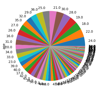
titanic.age.value_counts(dropna=True).plot.pie()
getting rid of nans
ages = pd.DataFrame()

ages['fillna(0)']      = titanic['age'].fillna(0)
ages['fillna - ffill'] = titanic['age'].fillna(method='ffill')
ages['fillna - bfill'] = titanic['age'].fillna(method='bfill')
ages['dropna']         = titanic['age'].dropna(inplace=False )
ages['interpolate']    = titanic['age'].interpolate()
ages['min']            = titanic['age'].fillna(titanic['age'].min())
ages['mean']           = titanic['age'].fillna(titanic['age'].mean())
ages[4:7]
|
fillna(0) |
fillna - ffill |
fillna - bfill |
dropna |
interpolate |
min |
mean |
| 4 |
35.0 |
35.0 |
35.0 |
35.0 |
35.0 |
35.00 |
35.000000 |
| 5 |
0.0 |
35.0 |
54.0 |
NaN |
44.5 |
0.42 |
29.699118 |
| 6 |
54.0 |
54.0 |
54.0 |
54.0 |
54.0 |
54.00 |
54.000000 |
#Melting/Mergin/Concating Data
titanic = pd.read_csv(url_titanic, keep_default_na=True)
titanic.head(3)
|
survived |
pclass |
sex |
age |
sibsp |
parch |
fare |
embarked |
class |
who |
adult_male |
deck |
embark_town |
alive |
alone |
| 0 |
0 |
3 |
male |
22.0 |
1 |
0 |
7.2500 |
S |
Third |
man |
True |
NaN |
Southampton |
no |
False |
| 1 |
1 |
1 |
female |
38.0 |
1 |
0 |
71.2833 |
C |
First |
woman |
False |
C |
Cherbourg |
yes |
False |
| 2 |
1 |
3 |
female |
26.0 |
0 |
0 |
7.9250 |
S |
Third |
woman |
False |
NaN |
Southampton |
yes |
True |
Renaming columns and indexes
titanic.rename(columns={'sex':'gender'}, inplace=True)
titanic.head(3)
|
survived |
pclass |
gender |
age |
sibsp |
parch |
fare |
embarked |
class |
who |
adult_male |
deck |
embark_town |
alive |
alone |
| 0 |
0 |
3 |
male |
22.0 |
1 |
0 |
7.2500 |
S |
Third |
man |
True |
NaN |
Southampton |
no |
False |
| 1 |
1 |
1 |
female |
38.0 |
1 |
0 |
71.2833 |
C |
First |
woman |
False |
C |
Cherbourg |
yes |
False |
| 2 |
1 |
3 |
female |
26.0 |
0 |
0 |
7.9250 |
S |
Third |
woman |
False |
NaN |
Southampton |
yes |
True |
droping columns
titanic.drop('embarked', axis=1, errors="ignore", inplace=True)
titanic.drop('who', axis=1, errors="ignore", inplace=True)
titanic.drop(['adult_male', 'alone'], axis=1, errors="ignore", inplace=True)
titanic.drop(['parch', 'deck'], axis=1, errors="ignore", inplace=True)
titanic.head(3)
|
survived |
pclass |
gender |
age |
sibsp |
fare |
class |
embark_town |
alive |
| 0 |
0 |
3 |
male |
22.0 |
1 |
7.2500 |
Third |
Southampton |
no |
| 1 |
1 |
1 |
female |
38.0 |
1 |
71.2833 |
First |
Cherbourg |
yes |
| 2 |
1 |
3 |
female |
26.0 |
0 |
7.9250 |
Third |
Southampton |
yes |
# fares
titanic = titanic.groupby(['class', 'embark_town', 'gender'])['age'].mean().reset_index()
titanic
|
class |
embark_town |
gender |
age |
| 0 |
First |
Cherbourg |
female |
36.052632 |
| 1 |
First |
Cherbourg |
male |
40.111111 |
| 2 |
First |
Queenstown |
female |
33.000000 |
| 3 |
First |
Queenstown |
male |
44.000000 |
| 4 |
First |
Southampton |
female |
32.704545 |
| 5 |
First |
Southampton |
male |
41.897188 |
| 6 |
Second |
Cherbourg |
female |
19.142857 |
| 7 |
Second |
Cherbourg |
male |
25.937500 |
| 8 |
Second |
Queenstown |
female |
30.000000 |
| 9 |
Second |
Queenstown |
male |
57.000000 |
| 10 |
Second |
Southampton |
female |
29.719697 |
| 11 |
Second |
Southampton |
male |
30.875889 |
| 12 |
Third |
Cherbourg |
female |
14.062500 |
| 13 |
Third |
Cherbourg |
male |
25.016800 |
| 14 |
Third |
Queenstown |
female |
22.850000 |
| 15 |
Third |
Queenstown |
male |
28.142857 |
| 16 |
Third |
Southampton |
female |
23.223684 |
| 17 |
Third |
Southampton |
male |
26.574766 |
pivoting data
titanic.pivot_table(index=['class','gender'],columns='embark_town',values='age').reset_index().head(3)
| embark_town |
class |
gender |
Cherbourg |
Queenstown |
Southampton |
| 0 |
First |
female |
36.052632 |
33.0 |
32.704545 |
| 1 |
First |
male |
40.111111 |
44.0 |
41.897188 |
| 2 |
Second |
female |
19.142857 |
30.0 |
29.719697 |
melting data
pd.melt(titanic, id_vars=['class', 'gender']).head(3)
|
class |
gender |
variable |
value |
| 0 |
First |
female |
embark_town |
Cherbourg |
| 1 |
First |
male |
embark_town |
Cherbourg |
| 2 |
First |
female |
embark_town |
Queenstown |
# todo - cover
# unstack()
# stack()
#Common Math operations over the DataFrames/Series
economics = pd.read_csv(url_economics, index_col='date',parse_dates=True)
economics.info()

> <class 'pandas.core.frame.DataFrame'>
> DatetimeIndex: 574 entries, 1967-07-01 to 2015-04-01
> Data columns (total 5 columns):
> #   Column    Non-Null Count  Dtype
> ---  ------    --------------  -----
> 0   pce       574 non-null    float64
> 1   pop       574 non-null    int64
> 2   psavert   574 non-null    float64
> 3   uempmed   574 non-null    float64
> 4   unemploy  574 non-null    int64
> dtypes: float64(3), int64(2)
> memory usage: 26.9 KB
|
pce |
pop |
psavert |
uempmed |
unemploy |
| count |
574.000000 |
574.000000 |
574.000000 |
574.000000 |
574.000000 |
| mean |
4843.510453 |
257189.381533 |
7.936585 |
8.610105 |
7771.557491 |
| std |
3579.287206 |
36730.801593 |
3.124394 |
4.108112 |
2641.960571 |
| min |
507.400000 |
198712.000000 |
1.900000 |
4.000000 |
2685.000000 |
| 25% |
1582.225000 |
224896.000000 |
5.500000 |
6.000000 |
6284.000000 |
| 50% |
3953.550000 |
253060.000000 |
7.700000 |
7.500000 |
7494.000000 |
| 75% |
7667.325000 |
290290.750000 |
10.500000 |
9.100000 |
8691.000000 |
| max |
12161.500000 |
320887.000000 |
17.000000 |
25.200000 |
15352.000000 |
economics.pce.mean()

result >>> 4843.510452961673
economics.pce = economics.pce * 2
economics.head()
|
pce |
pop |
psavert |
uempmed |
unemploy |
| date |
|
|
|
|
|
| 1967-07-01 |
1014.8 |
198712 |
12.5 |
4.5 |
2944 |
| 1967-08-01 |
1021.0 |
198911 |
12.5 |
4.7 |
2945 |
| 1967-09-01 |
1032.6 |
199113 |
11.7 |
4.6 |
2958 |
| 1967-10-01 |
1025.8 |
199311 |
12.5 |
4.9 |
3143 |
| 1967-11-01 |
1036.2 |
199498 |
12.5 |
4.7 |
3066 |
cs = economics.pce.cumsum()
ic(cs.head(1))
ic(cs.tail(1))

> ic> cs.head(1): date
> 1967-07-01    1014.8
> Name: pce, dtype: float64
> ic> cs.tail(1): date
> 2015-04-01    5560350.0
> Name: pce, dtype: float64

result >>> date
result >>> 2015-04-01    5560350.0
result >>> Name: pce, dtype: float64
#Math operations over the DataFrames/Series
Using aplly over column data
titanic = pd.read_csv(url_titanic, keep_default_na=True)
titanic.head(3)
|
survived |
pclass |
sex |
age |
sibsp |
parch |
fare |
embarked |
class |
who |
adult_male |
deck |
embark_town |
alive |
alone |
| 0 |
0 |
3 |
male |
22.0 |
1 |
0 |
7.2500 |
S |
Third |
man |
True |
NaN |
Southampton |
no |
False |
| 1 |
1 |
1 |
female |
38.0 |
1 |
0 |
71.2833 |
C |
First |
woman |
False |
C |
Cherbourg |
yes |
False |
| 2 |
1 |
3 |
female |
26.0 |
0 |
0 |
7.9250 |
S |
Third |
woman |
False |
NaN |
Southampton |
yes |
True |
def my_mean(vector):
    return vector * 5

titanic.rename(columns={'fare':'1912_£'}, inplace=True)
titanic['1912_$'] = titanic['1912_£'].apply(my_mean)

titanic.loc[:, ['class', '1912_£', '1912_$']].head(5)
|
class |
1912_£ |
1912_$ |
| 0 |
Third |
7.2500 |
36.2500 |
| 1 |
First |
71.2833 |
356.4165 |
| 2 |
Third |
7.9250 |
39.6250 |
| 3 |
First |
53.1000 |
265.5000 |
| 4 |
Third |
8.0500 |
40.2500 |
#Grouped Calculations
df = pd.read_csv(url_economics, parse_dates=['date'])
ic(df['date'].dtypes)

> ic> df['date'].dtypes: dtype('<M8[ns]')

result >>> dtype('<M8[ns]')
df.groupby('date')['pce', 'unemploy'].mean().head(10)

> /var/folders/7j/8x_gv0vs7f33q1cxc5cyhl3r0000gn/T/ipykernel_29394/3677347823.py:1: FutureWarning: Indexing with multiple keys (implicitly converted to a tuple of keys) will be deprecated, use a list instead.
> df.groupby('date')['pce', 'unemploy'].mean().head(10)
|
pce |
unemploy |
| date |
|
|
| 1967-07-01 |
507.4 |
2944.0 |
| 1967-08-01 |
510.5 |
2945.0 |
| 1967-09-01 |
516.3 |
2958.0 |
| 1967-10-01 |
512.9 |
3143.0 |
| 1967-11-01 |
518.1 |
3066.0 |
| 1967-12-01 |
525.8 |
3018.0 |
| 1968-01-01 |
531.5 |
2878.0 |
| 1968-02-01 |
534.2 |
3001.0 |
| 1968-03-01 |
544.9 |
2877.0 |
| 1968-04-01 |
544.6 |
2709.0 |
df.groupby(by=df['date'].dt.strftime('%Y'))['unemploy', 'uempmed'].mean().reset_index().head(3)

> /var/folders/7j/8x_gv0vs7f33q1cxc5cyhl3r0000gn/T/ipykernel_29394/1916814624.py:1: FutureWarning: Indexing with multiple keys (implicitly converted to a tuple of keys) will be deprecated, use a list instead.
> df.groupby(by=df['date'].dt.strftime('%Y'))['unemploy', 'uempmed'].mean().reset_index().head(3)
|
date |
unemploy |
uempmed |
| 0 |
1967 |
3012.333333 |
4.700000 |
| 1 |
1968 |
2797.416667 |
4.500000 |
| 2 |
1969 |
2830.166667 |
4.441667 |
df.groupby(by=df['date'].dt.strftime('%Y'))['unemploy', 'uempmed'].first().reset_index().head(3)

> /var/folders/7j/8x_gv0vs7f33q1cxc5cyhl3r0000gn/T/ipykernel_29394/2747298252.py:1: FutureWarning: Indexing with multiple keys (implicitly converted to a tuple of keys) will be deprecated, use a list instead.
> df.groupby(by=df['date'].dt.strftime('%Y'))['unemploy', 'uempmed'].first().reset_index().head(3)
|
date |
unemploy |
uempmed |
| 0 |
1967 |
2944 |
4.5 |
| 1 |
1968 |
2878 |
5.1 |
| 2 |
1969 |
2718 |
4.4 |
df.groupby(by=df['date'].dt.strftime('%Y'))['unemploy', 'uempmed'].last().reset_index().head(3)

> /var/folders/7j/8x_gv0vs7f33q1cxc5cyhl3r0000gn/T/ipykernel_29394/3124120651.py:1: FutureWarning: Indexing with multiple keys (implicitly converted to a tuple of keys) will be deprecated, use a list instead.
> df.groupby(by=df['date'].dt.strftime('%Y'))['unemploy', 'uempmed'].last().reset_index().head(3)
|
date |
unemploy |
uempmed |
| 0 |
1967 |
3018 |
4.8 |
| 1 |
1968 |
2685 |
4.4 |
| 2 |
1969 |
2884 |
4.6 |
#Joins
size = 6
df_square = pd.DataFrame(rnd.randint(0, 10, size**2).reshape(size, -1),
                  index=[f"R{x:02d}" for x in range(size)],
                  columns = [f"C{x:02d}" for x in range(size)])

df_square
|
C00 |
C01 |
C02 |
C03 |
C04 |
C05 |
| R00 |
2 |
6 |
5 |
7 |
8 |
4 |
| R01 |
0 |
2 |
9 |
7 |
5 |
7 |
| R02 |
8 |
3 |
0 |
0 |
9 |
3 |
| R03 |
6 |
1 |
2 |
0 |
4 |
0 |
| R04 |
7 |
0 |
0 |
1 |
1 |
5 |
| R05 |
6 |
4 |
0 |
0 |
2 |
1 |
df_line = pd.Series(rnd.randint(0, 10, size), index=[f"R{x+3:02d}" for x in range(size)])
df_line.name="C06"
df_line

result >>> R03    4
result >>> R04    9
result >>> R05    5
result >>> R06    6
result >>> R07    3
result >>> R08    6
result >>> Name: C06, dtype: int64
df_square['C06'] = df_line
df_square
|
C00 |
C01 |
C02 |
C03 |
C04 |
C05 |
C06 |
| R00 |
2 |
6 |
5 |
7 |
8 |
4 |
NaN |
| R01 |
0 |
2 |
9 |
7 |
5 |
7 |
NaN |
| R02 |
8 |
3 |
0 |
0 |
9 |
3 |
NaN |
| R03 |
6 |
1 |
2 |
0 |
4 |
0 |
4.0 |
| R04 |
7 |
0 |
0 |
1 |
1 |
5 |
9.0 |
| R05 |
6 |
4 |
0 |
0 |
2 |
1 |
5.0 |
clean up data
df_square.drop('C06', axis=1, errors="ignore", inplace=True)
df_square.join(pd.DataFrame(df_line), how="inner")
|
C00 |
C01 |
C02 |
C03 |
C04 |
C05 |
C06 |
| R03 |
6 |
1 |
2 |
0 |
4 |
0 |
4 |
| R04 |
7 |
0 |
0 |
1 |
1 |
5 |
9 |
| R05 |
6 |
4 |
0 |
0 |
2 |
1 |
5 |
df_square.join(pd.DataFrame(df_line), how="outer")
|
C00 |
C01 |
C02 |
C03 |
C04 |
C05 |
C06 |
| R00 |
2.0 |
6.0 |
5.0 |
7.0 |
8.0 |
4.0 |
NaN |
| R01 |
0.0 |
2.0 |
9.0 |
7.0 |
5.0 |
7.0 |
NaN |
| R02 |
8.0 |
3.0 |
0.0 |
0.0 |
9.0 |
3.0 |
NaN |
| R03 |
6.0 |
1.0 |
2.0 |
0.0 |
4.0 |
0.0 |
4.0 |
| R04 |
7.0 |
0.0 |
0.0 |
1.0 |
1.0 |
5.0 |
9.0 |
| R05 |
6.0 |
4.0 |
0.0 |
0.0 |
2.0 |
1.0 |
5.0 |
| R06 |
NaN |
NaN |
NaN |
NaN |
NaN |
NaN |
6.0 |
| R07 |
NaN |
NaN |
NaN |
NaN |
NaN |
NaN |
3.0 |
| R08 |
NaN |
NaN |
NaN |
NaN |
NaN |
NaN |
6.0 |
df_square.join(pd.DataFrame(df_line), how="left")
|
C00 |
C01 |
C02 |
C03 |
C04 |
C05 |
C06 |
| R00 |
2 |
6 |
5 |
7 |
8 |
4 |
NaN |
| R01 |
0 |
2 |
9 |
7 |
5 |
7 |
NaN |
| R02 |
8 |
3 |
0 |
0 |
9 |
3 |
NaN |
| R03 |
6 |
1 |
2 |
0 |
4 |
0 |
4.0 |
| R04 |
7 |
0 |
0 |
1 |
1 |
5 |
9.0 |
| R05 |
6 |
4 |
0 |
0 |
2 |
1 |
5.0 |
df_square.join(pd.DataFrame(df_line), how="right")
|
C00 |
C01 |
C02 |
C03 |
C04 |
C05 |
C06 |
| R03 |
6.0 |
1.0 |
2.0 |
0.0 |
4.0 |
0.0 |
4 |
| R04 |
7.0 |
0.0 |
0.0 |
1.0 |
1.0 |
5.0 |
9 |
| R05 |
6.0 |
4.0 |
0.0 |
0.0 |
2.0 |
1.0 |
5 |
| R06 |
NaN |
NaN |
NaN |
NaN |
NaN |
NaN |
6 |
| R07 |
NaN |
NaN |
NaN |
NaN |
NaN |
NaN |
3 |
| R08 |
NaN |
NaN |
NaN |
NaN |
NaN |
NaN |
6 |
#Sorting values and indexes
economics = pd.read_csv(url_economics, index_col='date',parse_dates=True)
economics.sort_values(by='unemploy', ascending=False).head(3)
|
pce |
pop |
psavert |
uempmed |
unemploy |
| date |
|
|
|
|
|
| 2009-10-01 |
9924.6 |
308189 |
5.4 |
18.9 |
15352 |
| 2010-04-01 |
10106.9 |
309191 |
5.6 |
22.1 |
15325 |
| 2009-11-01 |
9946.1 |
308418 |
5.7 |
19.8 |
15219 |
economics.sort_index(ascending=False).head(3)
|
pce |
pop |
psavert |
uempmed |
unemploy |
| date |
|
|
|
|
|
| 2015-04-01 |
12158.9 |
320887 |
5.6 |
11.7 |
8549 |
| 2015-03-01 |
12161.5 |
320707 |
5.2 |
12.2 |
8575 |
| 2015-02-01 |
12095.9 |
320534 |
5.7 |
13.1 |
8705 |
#Time Series Analisis
economics = pd.read_csv(url_economics, index_col='date',parse_dates=True)
economics.head(2)
|
pce |
pop |
psavert |
uempmed |
unemploy |
| date |
|
|
|
|
|
| 1967-07-01 |
507.4 |
198712 |
12.5 |
4.5 |
2944 |
| 1967-08-01 |
510.5 |
198911 |
12.5 |
4.7 |
2945 |
economics.index

result >>> DatetimeIndex(['1967-07-01', '1967-08-01', '1967-09-01', '1967-10-01',
result >>>                '1967-11-01', '1967-12-01', '1968-01-01', '1968-02-01',
result >>>                '1968-03-01', '1968-04-01',
result >>>                ...
result >>>                '2014-07-01', '2014-08-01', '2014-09-01', '2014-10-01',
result >>>                '2014-11-01', '2014-12-01', '2015-01-01', '2015-02-01',
result >>>                '2015-03-01', '2015-04-01'],
result >>>               dtype='datetime64[ns]', name='date', length=574, freq=None)
TIME SERIES OFFSET ALIASES
| ALIAS |
DESCRIPTION |
| B |
business day frequency |
| C |
custom business day frequency (experimental) |
| D |
calendar day frequency |
| W |
weekly frequency |
| M |
month end frequency |
| SM |
semi-month end frequency (15th and end of month) |
| BM |
business month end frequency |
| CBM |
custom business month end frequency |
| MS |
month start frequency |
| SMS |
semi-month start frequency (1st and 15th) |
| BMS |
business month start frequency |
| CBMS |
custom business month start frequency |
| Q |
quarter end frequency |
| BQ |
business quarter endfrequency |
| QS |
quarter start frequency |
| BQS |
business quarter start frequency |
| A |
year end frequency |
| BA |
business year end frequency |
| AS |
year start frequency |
| BAS |
business year start frequency |
| BH |
business hour frequency |
| H |
hourly frequency |
| T, min |
minutely frequency |
| S |
secondly frequency |
| L, ms |
milliseconds |
| U, us |
microseconds |
| N |
nanoseconds |
#Time Resampling
# yearly
economics.resample(rule='A').mean().head(3)
|
pce |
pop |
psavert |
uempmed |
unemploy |
| date |
|
|
|
|
|
| 1967-12-31 |
515.166667 |
199200.333333 |
12.300000 |
4.700000 |
3012.333333 |
| 1968-12-31 |
557.458333 |
200663.750000 |
11.216667 |
4.500000 |
2797.416667 |
| 1969-12-31 |
604.483333 |
202648.666667 |
10.741667 |
4.441667 |
2830.166667 |
economics.resample(rule='A').first().head(3)
|
pce |
pop |
psavert |
uempmed |
unemploy |
| date |
|
|
|
|
|
| 1967-12-31 |
507.4 |
198712 |
12.5 |
4.5 |
2944 |
| 1968-12-31 |
531.5 |
199808 |
11.7 |
5.1 |
2878 |
| 1969-12-31 |
584.2 |
201760 |
10.0 |
4.4 |
2718 |
# custom resampling function

def total(entry):
    if len(entry):
        return entry.sum()

economics.unemploy.resample(rule='A').apply(total).head(2)

result >>> date
result >>> 1967-12-31    18074
result >>> 1968-12-31    33569
result >>> Freq: A-DEC, Name: unemploy, dtype: int64
#Time/Data Shifting
http://pandas.pydata.org/pandas-docs/stable/generated/pandas.DataFrame.shift.html
economics.unemploy.shift(1).head(2)

result >>> date
result >>> 1967-07-01       NaN
result >>> 1967-08-01    2944.0
result >>> Name: unemploy, dtype: float64
# Shift everything forward one month
economics.unemploy.shift(periods=2, freq='M').head()

result >>> date
result >>> 1967-08-31    2944
result >>> 1967-09-30    2945
result >>> 1967-10-31    2958
result >>> 1967-11-30    3143
result >>> 1967-12-31    3066
result >>> Name: unemploy, dtype: int64
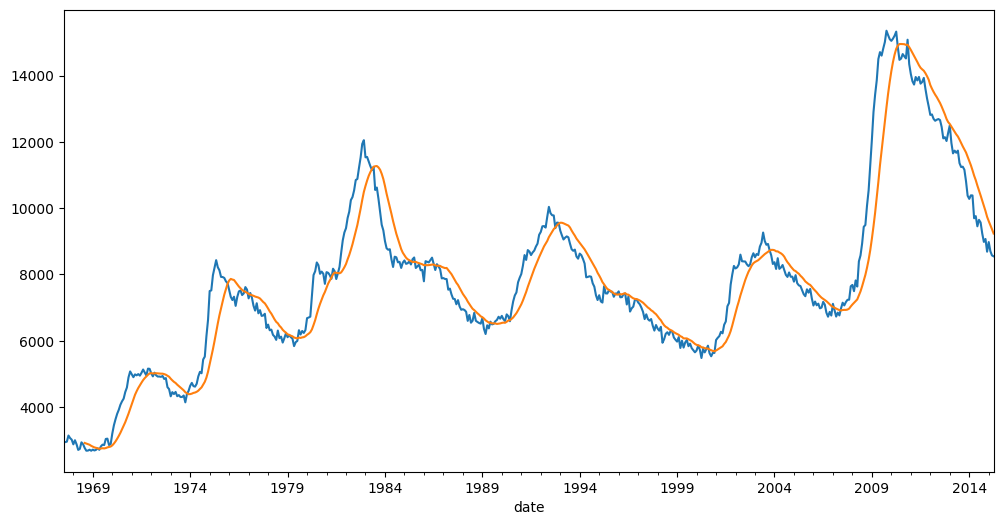
#Rolling and Expanding
A common process with time series is to create data based off of a rolling mean. The idea is to divide the data into “windows” of time, and then calculate an aggregate function for each window. In this way we obtain a simple moving average.
economics.unemploy.plot(figsize=(12,6)).autoscale(axis='x',tight=True)
economics.unemploy.rolling(window=14).mean().plot()
# economics.unemploy.rolling(window=30).max().plot()
# economics.unemploy.rolling(window=30).min().plot()
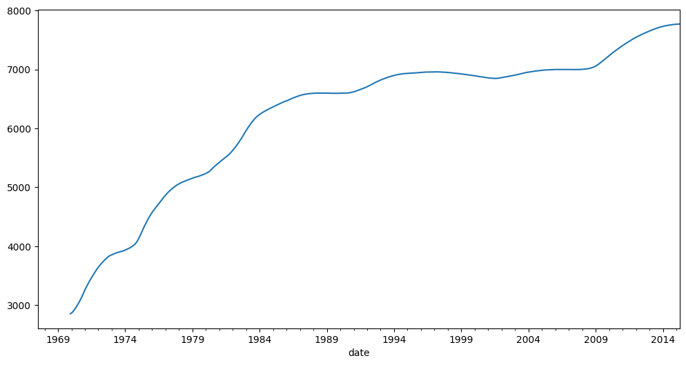
Instead of calculating values for a rolling window of dates, what if you wanted to take into account everything from the start of the time series up to each point in time? For example, instead of considering the average over the last 7 days, we would consider all prior data in our expanding set of averages.
economics.unemploy.expanding(min_periods=30).mean().plot(figsize=(12,6))
#Visualization
import matplotlib.pyplot as plt
%matplotlib inline
economics = pd.read_csv(url_economics, index_col='date',parse_dates=True)
economics.head(2)
|
pce |
pop |
psavert |
uempmed |
unemploy |
| date |
|
|
|
|
|
| 1967-07-01 |
507.4 |
198712 |
12.5 |
4.5 |
2944 |
| 1967-08-01 |
510.5 |
198911 |
12.5 |
4.7 |
2945 |
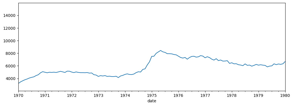
# ploting all data for a range of x values (date index)
_ = economics.unemploy.plot(
    figsize=(12,4),
    xlim=['1970', '1980'],
)
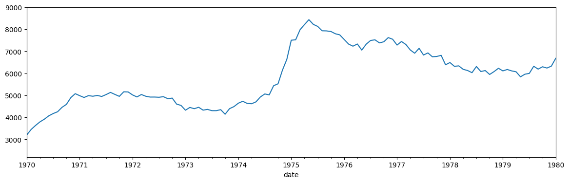
# or we can specify what column we want to plot
ax = economics['unemploy'].plot(
    figsize=(14,4),
    xlim=['1970', '1980'],
    ylim=[2200, 9000],
    title="Unemployment for period 1970-1980"
)
_ = ax.set(ylabel="Unemployment", xlabel="Years")

# this will make data to fit, no matter what we set in x
# ax.autoscale(axis='x',tight=True)

# x as slicing
economics['unemploy']['1970':'1979'].plot(figsize=(14,4), ls='--',c='r').autoscale(axis='x',tight=True)

# or providing argument
_ = economics['unemploy'].plot(figsize=(14,4), xlim=['1970','1980'], ylim=[2200, 9000])
#X-Ticks
https://matplotlib.org/api/dates_api.html
Formatting follows the Python datetime strftime codes.
The following examples are based on datetime.datetime(2001, 2, 3, 16, 5, 6) :
| CODE |
MEANING |
EXAMPLE |
%Y |
Year with century as a decimal number |
2001 |
%y |
Year without century as a zero-padded decimal number |
01 |
%m |
Month as a zero-padded decimal number |
02 |
%B |
Month as locale’s full name |
February |
%b |
Month as locale’s abbreviated name |
Feb |
%d |
Day of the month as a zero-padded decimal number |
03 |
%A |
Weekday as locale’s full name |
Saturday |
%a |
Weekday as locale’s abbreviated name |
Sat |
%H |
Hour (24-hour clock) as a zero-padded decimal number |
16 |
%I |
Hour (12-hour clock) as a zero-padded decimal number |
04 |
%p |
Locale’s equivalent of either AM or PM |
PM |
%M |
Minute as a zero-padded decimal number |
05 |
%S |
Second as a zero-padded decimal number |
06 |
| CODE |
MEANING |
EXAMPLE |
%#m |
Month as a decimal number. (Windows) |
2 |
%-m |
Month as a decimal number. (Mac/Linux) |
2 |
%#x |
Long date |
Saturday, February 03, 2001 |
%#c |
Long date and time |
Saturday, February 03, 2001 16:05:06 |
from datetime import datetime
datetime(2001, 2, 3, 16, 5, 6).strftime("%A, %B %d, %Y  %I:%M:%S %p")

result >>> 'Saturday, February 03, 2001  04:05:06 PM'
from matplotlib import dates
# TODO - find better example so i can use month or weekend formatter.
# using Date Locator's
#Miscellaneous
#Loops
# series
s = pd.Series(range(10000))
# list
l = list(s)
Panda’s Time Series
%timeit -n 1 -r 1 [s.iloc[i] for i in range(len(s))]

> 21.4 ms ± 0 ns per loop (mean ± std. dev. of 1 run, 1 loop each)
Python’s list
%timeit -n 1 -r 1 [l[i] for i in range(len(l))]

> 189 µs ± 0 ns per loop (mean ± std. dev. of 1 run, 1 loop each)
Pandas - accesing lst element
%timeit -n 1 -r 1 s.iloc[-1:]

> 53.8 µs ± 0 ns per loop (mean ± std. dev. of 1 run, 1 loop each)
List - accesing lst element
%timeit -n 1 -r 1 l[-1:]

> 375 ns ± 0 ns per loop (mean ± std. dev. of 1 run, 1 loop each)