Statistical Distributions

%matplotlib inline
import pandas as pd
import numpy as np
import scipy.stats as stats
import matplotlib.pyplot as plt

plt.rcParams.update({
    'font.size': 20.0, 
    'axes.titlesize': 'small', 
    'axes.labelsize': 'small', 
    'xtick.labelsize': 'small', 
    'ytick.labelsize': 'small'
})

def plot_continuous(dist):
    fig, ax = plt.subplots(1, 2, sharex=True, figsize=(15, 5))
    # Plot hist
    rvs = dist.rvs(size=1000) 
     
    ax[0].hist(rvs, alpha=0.2, histtype='stepfilled')
    x=np.linspace(dist.ppf(0.01), dist.ppf(0.99), 50) 
    ax[0].plot(x, dist.pdf(x), '-', lw=2);
    ax[0].set_title( dist.dist.name.title() + ' PDF') 
    ax[0].set_ylabel('p(X=x)')
    
    # Plot cdf.
    ax[1].plot(x, dist.cdf(x), '-', lw=2) 
    ax[1].set_title( dist.dist.name.title() + ' CDF') 
    ax[1].set_ylabel('p(X<=x)') 
    ax[1].set_xlabel('x');
    return (fig, ax)  


def plot_discrete(dist):
    fig, ax = plt.subplots(1, 2, sharex=True, figsize=(15, 5))
    
    # Plot hist
    rvs = dist.rvs(size=1000)
    w = np.ones_like(rvs)/ float(len(rvs))
    ax[0].hist(rvs, weights=w, alpha=0.2, histtype='stepfilled')
    
    # Plot pmf.
    k = np.arange(dist.ppf(0.01), dist.ppf(0.99)+1)
    ax[0].plot(k, dist.pmf(k), 'bo', lw=2);
    ax[0].set_title( dist.dist.name.title() + ' PMF') 
    ax[0].set_ylabel('p(X=k)')

    # Plot cdf.
    ax[1].plot(k, dist.cdf(k), 'bo', lw=2);
    ax[1].set_title( dist.dist.name.title() + ' CDF') 
    ax[1].set_ylabel('p(X<=k)') 
    ax[1].set_xlabel('k');
    return (fig, ax)

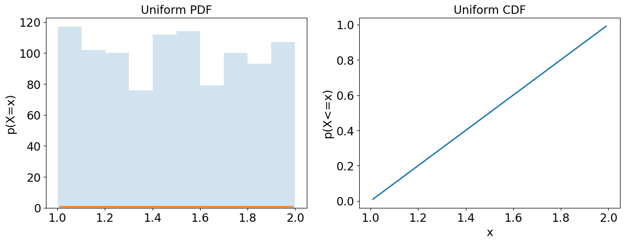
Uniform (Continuous)

#Models

Equally likely outcomes in the interval a to b, e.g. degrees between hour and minute hand.

#Parameters

a minimum value.
b maximum value.
x observed value.

a,b = 1,2
uniform = stats.uniform(loc=a, scale=b-a) 
plot = plot_continuous(uniform)

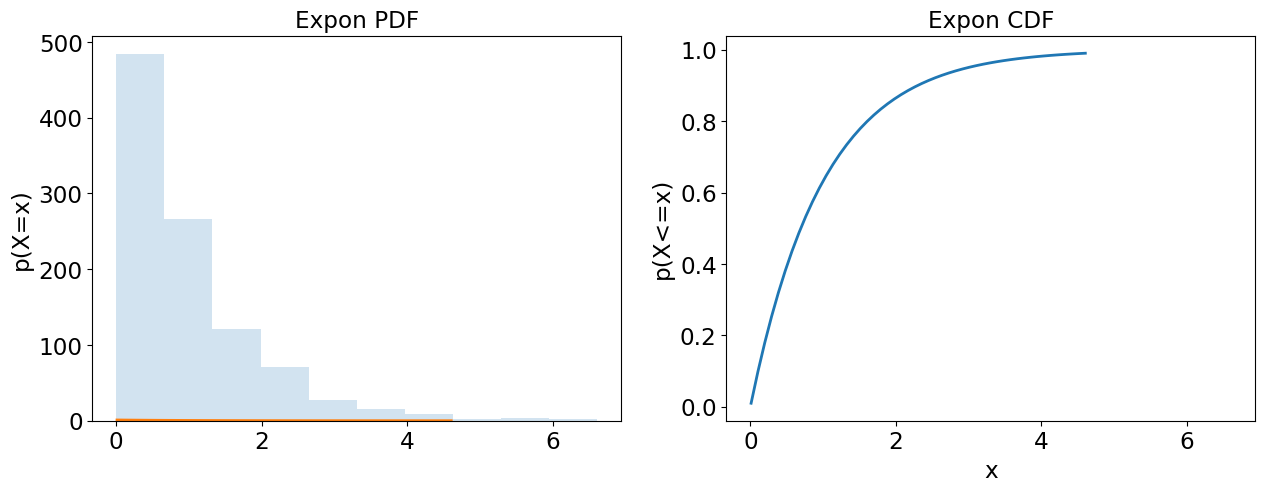
Exponential (Continuous)

#Models

Time between poisson events, e.g. time until taxi will pass street corner.

#Parameters

lambda average number of independent events per interval.
x observed time between events.

lam = 1  # lambda
exponential = stats.expon(scale=1/lam) 
plot = plot_continuous(exponential)

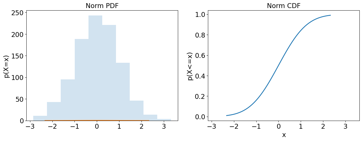
Gaussian (Continuous)

#Models

A bell curve, e.g. IQ score.

#Parameters

mu mean or expectation.
sigma standard deviation.
x observed value.

mu, sigma = 0, 1 
gaussian=stats.norm(loc=mu,scale=sigma) 
plot = plot_continuous(gaussian)

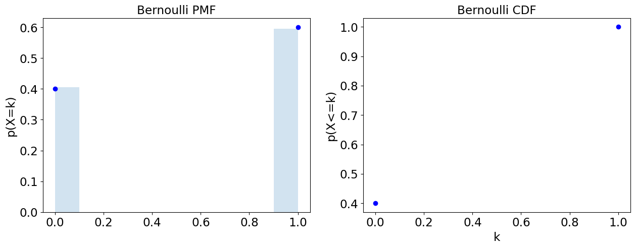
Bernoulli (Discrete)

#Models

One instance of a success or failure trial, e.g. (possibly unfair) coin toss.

#Parameters

p probability of success.
k failure or success, i.e. {0,1}, observation.

bernoulli = stats.bernoulli(p=0.6) 
plot = plot_discrete(bernoulli)

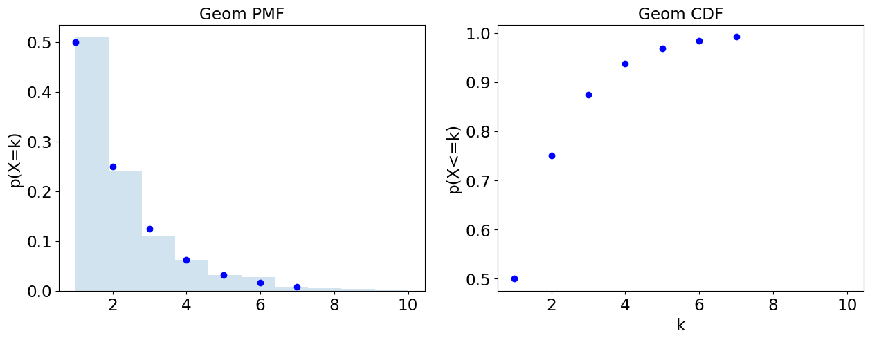
Geometric (Discrete)

#Models

Number of Bernoulli trials until first success, e.g. number of trials until coin flip turns out to be heads.

#Parameters

p probability of success (each trial).
k observed trials until success.

geometric = stats.geom(p=0.5) 
plot = plot_discrete(geometric)

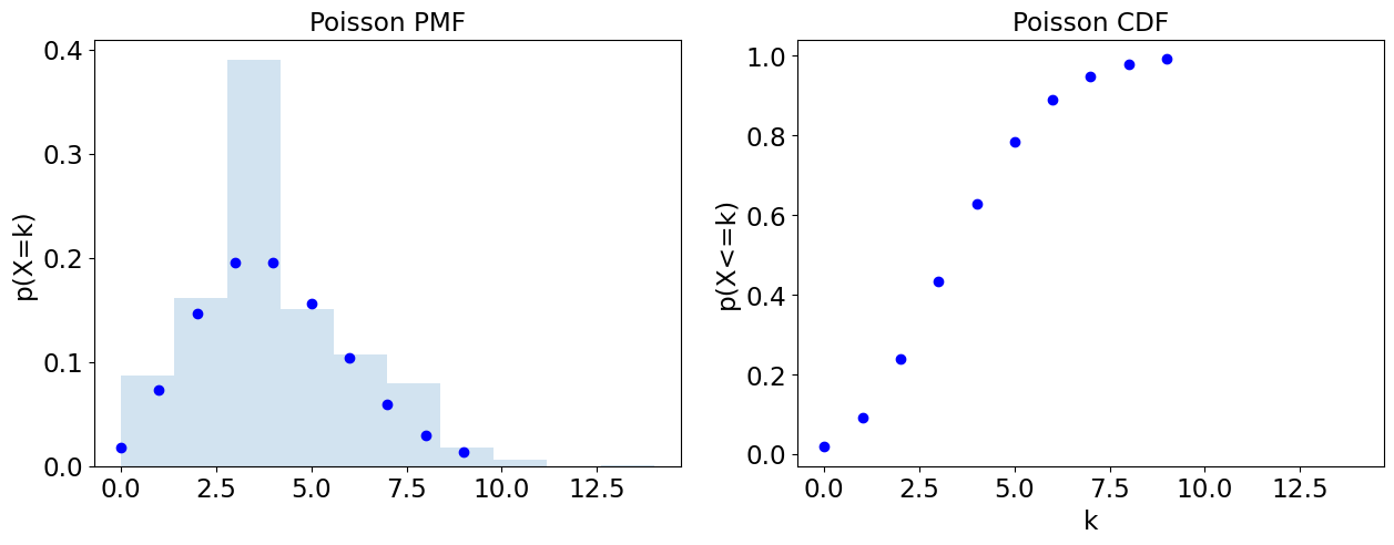
Poisson (Discrete)

#Models

Number of events occurring in a fixed interval, e.g. number of taxis passing a street corner in a given hour (on avg. 10/hr).

#Parameters

lambda average number of independent events per interval.
k events observed in an interval.

lam = 4  # lambda
poisson = stats.poisson(mu=lam) 
plot = plot_discrete(poisson)

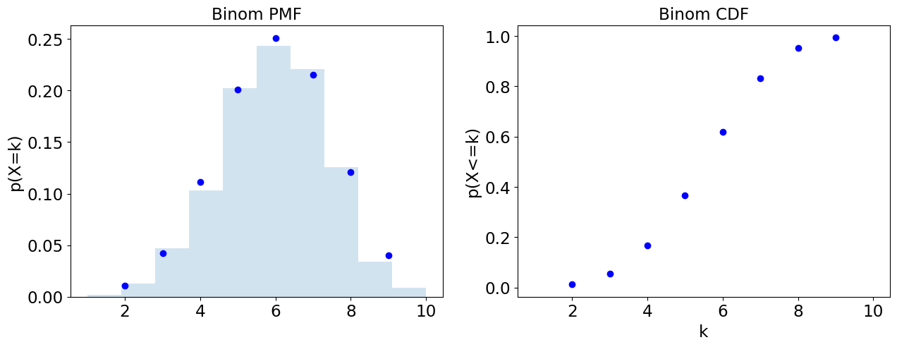
Binomial (Discrete)

#Models

Number of successes out of a number of Bernoulli trials with replacement., e.g. number of coin flips out of 100 that turn out to be heads.

#Parameters:

p probability of success (each trial).
n number of independent trials.
k observed number of successes

binomial=stats.binom(n=10,p=0.6); 
plot = plot_discrete(binomial)

Weibull (Continuous)

#Models

Time between events when rate is not constant, e.g. time-to-failure when rate of failure increases or decreases over time.

Gamma (Continuous)

#Models

Waiting time between Poisson distributed events. Used when waiting times between events are relevant, e.g. aggregate insurance claims or the amount of rainfall accumulated in a reservoir.

Hypergeometric (Discrete)

#Models

Number of successes out of a number of success or failure trials without replacement, e.g. Number of times you draw a black ball from an urn of black and white balls without putting any back.